Reading VCFs and Building Mutational-Spectrum Catalogs
Source:vignettes/mSigSpectra.Rmd
mSigSpectra.RmdThis vignette walks through the four-step
mSigSpectra pipeline — read_vcf →
split_vcf → annotate_sbs_or_dbs_vcf /
annotate_id_vcf → vcf_to_sbs_catalog /
vcf_to_dbs_catalog / vcf_to_id_catalog — using
a real Strelka VCF that ships with the package. It then plots each
catalog with mSigPlot.
If you do not have the BSgenome package or mSigPlot
installed, the chunks below will be skipped at render time. To
install:
BiocManager::install("BSgenome.Hsapiens.1000genomes.hs37d5")
remotes::install_github("steverozen/mSigPlot")
1. Load packages
library(mSigSpectra)
library(mSigPlot)
#>
#> Attaching package: 'mSigPlot'
#> The following object is masked from 'package:mSigSpectra':
#>
#>     catalog_row_order
2. Locate test VCFs
Three example VCFs ship with the package: a Strelka SBS file, a Strelka indel file, and a Mutect file (all small subsets, GRCh37 / hg19).
sbs_file <- system.file(
  "extdata", "Strelka-SBS-GRCh37", "Strelka.SBS.GRCh37.s1.vcf",
  package = "mSigSpectra"
)
id_file <- system.file(
  "extdata", "Strelka-ID-GRCh37", "Strelka.ID.GRCh37.s1.vcf",
  package = "mSigSpectra"
)
mutect_file <- system.file(
  "extdata", "Mutect-GRCh37", "Mutect.GRCh37.s1.vcf",
  package = "mSigSpectra"
)
3. Read the SBS VCF
read_vcf() returns a data.table with
whatever columns the VCF body contains. We pass
filter = "PASS" to match the Strelka convention.
sbs_vcf <- read_vcf(sbs_file, filter = "PASS")
nrow(sbs_vcf)
#> [1] 798
head(sbs_vcf[, c("CHROM", "POS", "REF", "ALT", "FILTER")])
#>     CHROM     POS    REF    ALT FILTER
#>    <char>   <int> <char> <char> <char>
#> 1:      1  906904      C      A   PASS
#> 2:      1 1821952      C      T   PASS
#> 3:      1 1963733      G      A   PASS
#> 4:      1 2249474      G      T   PASS
#> 5:      1 2545983      A      T   PASS
#> 6:      1 2738084      C      A   PASS
4. Split into SBS / DBS / ID sub-tables
split_vcf() partitions rows by
REF/ALT length alone. For a “pure SBS” VCF you
would expect everything in $SBS, but Strelka’s SBS caller
can emit adjacent SBS pairs that the indel caller does not see;
mSigSpectra does not merge them into DBSs (see
“Gotchas” in the README) — they stay as SBSs.
5. Annotate the SBS rows
annotate_sbs_or_dbs_vcf() adds:
-
seq.<N>bases— the flanking sequence context (defaultseq.21bases). - For ref genomes with a shipped transcript-ranges table (GRCh37 /
GRCh38 / GRCm38), the transcript-strand columns
trans.start.pos,trans.end.pos,trans.strand,trans.Ensembl.gene.ID,trans.gene.symbol, plusbothstrandandcount(number of overlapping transcripts).
It returns a list with annotated.vcf (the table below)
and discarded.variants (always NULL for SBS /
DBS).
sbs_ann <- annotate_sbs_or_dbs_vcf(sbs_split$SBS,
                                   ref_genome = "GRCh37")$annotated.vcf
new_cols <- setdiff(colnames(sbs_ann), colnames(sbs_split$SBS))
new_cols
#> [1] "seq.21bases"           "trans.start.pos"       "trans.end.pos"
#> [4] "trans.strand"          "trans.Ensembl.gene.ID" "trans.gene.symbol"
#> [7] "POS2"                  "bothstrand"            "count"
6. Build SBS catalogs
A catalog is a single-column numeric matrix with attributes (no S3 class). One call per resolution.
cat96 <- vcf_to_sbs_catalog(sbs_ann, type = "SBS96", ref_genome = "GRCh37",
                            region = "genome", sample_name = "s1")
cat192 <- vcf_to_sbs_catalog(sbs_ann, type = "SBS192", ref_genome = "GRCh37",
                             region = "transcript", sample_name = "s1")
cat1536 <- vcf_to_sbs_catalog(sbs_ann, type = "SBS1536", ref_genome = "GRCh37",
                              region = "genome", sample_name = "s1")

dim(cat96)
#> [1] 96  1
sum(cat96)
#> [1] 798
catalog_attrs(cat96)
#> $type
#> [1] "SBS96"
#>
#> $counts_or_density
#> [1] "counts"
#>
#> $ref_genome
#> | BSgenome object for Human
#> | - organism: Homo sapiens
#> | - provider: 1000genomes
#> | - genome: hs37d5
#> | - release date: 2011-07-07
#> | - 86 sequence(s):
#> |     1          2          3          4          5          6
#> |     7          8          9          10         11         12
#> |     13         14         15         16         17         18
#> |     19         20         21         22         X          Y
#> |     MT         GL000207.1 GL000226.1 GL000229.1 GL000231.1 GL000210.1
#> |     ...        ...        ...        ...        ...        ...
#> |     GL000228.1 GL000214.1 GL000221.1 GL000209.1 GL000218.1 GL000220.1
#> |     GL000213.1 GL000211.1 GL000199.1 GL000217.1 GL000216.1 GL000215.1
#> |     GL000205.1 GL000219.1 GL000224.1 GL000223.1 GL000195.1 GL000212.1
#> |     GL000222.1 GL000200.1 GL000193.1 GL000194.1 GL000225.1 GL000192.1
#> |     NC_007605  hs37d5
#> |
#> | Tips: call 'seqnames()' on the object to get all the sequence names, call
#> | 'seqinfo()' to get the full sequence info, use the '$' or '[[' operator to
#> | access a given sequence, see '?BSgenome' for more information.
#>
#> $region
#> [1] "genome"
#>
#> $abundance
#>       TTT       GTT       CTT       ATT       ACA       ACC       ACG       ACT
#> 142250238  78687790 107617082 129934569 108258537  64600793  14067800  89401111
#>       TCT       GCT       CCT       ATA       ATC       ATG       TTG       GTG
#> 120134425  78722685  98950493 108767627  74496273 102345885 101674674  82782961
#>       CTG       CCA       CCC       CCG       TCG       GCG       CTA       CTC
#> 114948303 102519417  64749177  15301553  12406623  13282321  71873805  94271285
#>       TTC       GTC       GCA       GCC       TCC       GTA       TTA       TCA
#> 106058961  53511169  81041806  66773820  85103213  63617716 108282800 108631566
7. Plot SBS catalogs
plot_SBS96(cat96, plot_title = "Strelka.SBS.GRCh37.s1 — SBS96")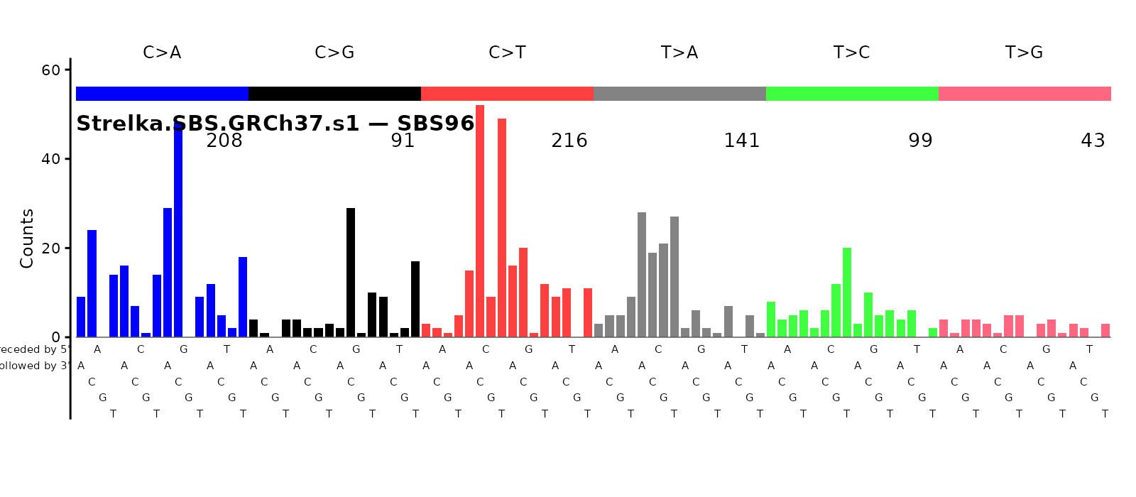
plot_SBS192(cat192, plot_title = "Strelka.SBS.GRCh37.s1 — SBS192 (stranded)")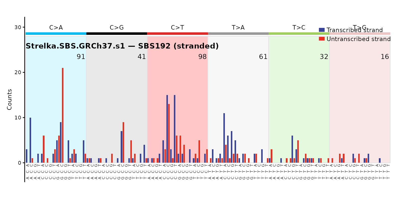
plot_SBS1536(cat1536, plot_title = "Strelka.SBS.GRCh37.s1 — SBS1536")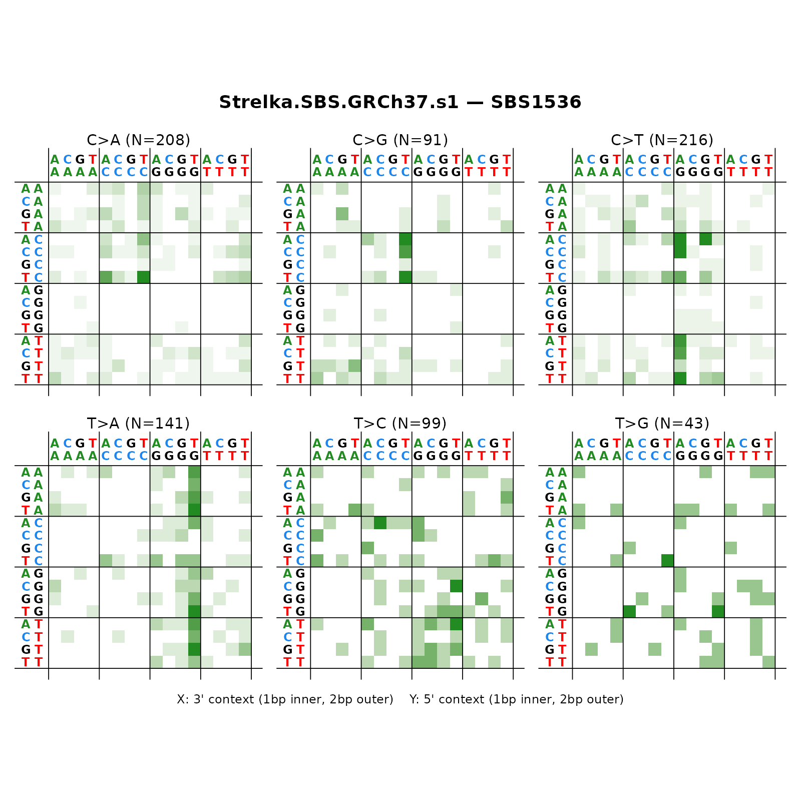
8. Build and plot ID catalogs
The Strelka indel VCF goes through annotate_id_vcf(),
which left-justifies each indel, extracts the local repeat /
microhomology context, and emits the three classification strings
(COSMIC_83, Koh_89, Koh_476).
Like annotate_sbs_or_dbs_vcf() it returns a list of
annotated.vcf + discarded.variants.
id_vcf <- read_vcf(id_file, filter = "PASS")
id_split <- split_vcf(id_vcf, name_of_vcf = "Strelka.ID.GRCh37.s1")
id_ann <- annotate_id_vcf(id_split$ID,
                          ref_genome = "GRCh37")$annotated.vcf
id_ann[1, c("CHROM", "POS", "REF", "ALT", "COSMIC_83", "Koh_89")]
#>     CHROM     POS    REF    ALT COSMIC_83       Koh_89
#>    <char>   <int> <char> <char>    <char>       <char>
#> 1:      1 5288645     TG      T DEL:C:1:1 [Del(C):R2]A

cat_id83 <- vcf_to_id_catalog(id_ann, type = "ID83", ref_genome = "GRCh37",
                              region = "genome", sample_name = "s1")
cat_id89 <- vcf_to_id_catalog(id_ann, type = "ID89", ref_genome = "GRCh37",
                              region = "genome", sample_name = "s1")
cat_id476 <- vcf_to_id_catalog(id_ann, type = "ID476", ref_genome = "GRCh37",
                               region = "genome", sample_name = "s1")
plot_ID83(cat_id83, plot_title = "Strelka.ID.GRCh37.s1 — ID83")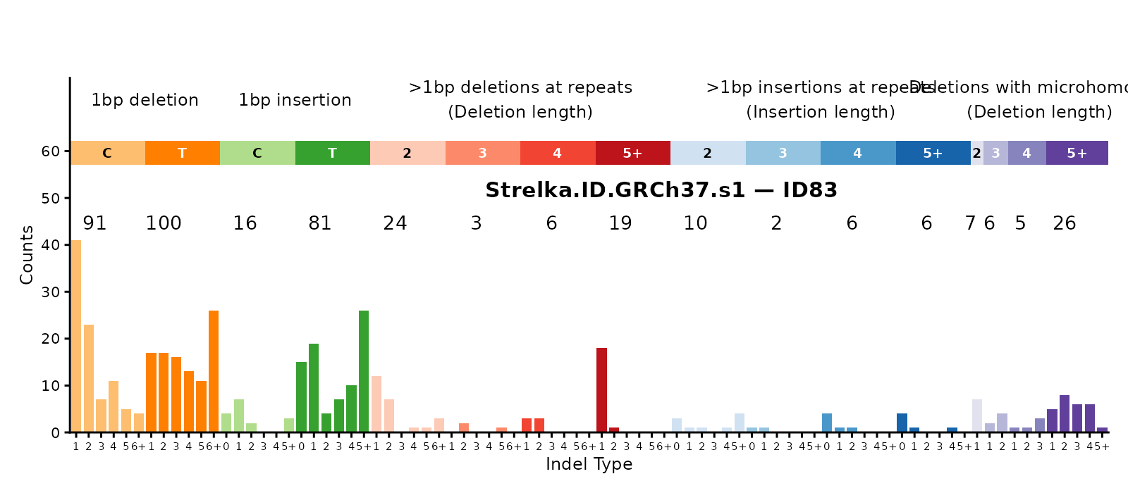
plot_ID89(cat_id89, plot_title = "Strelka.ID.GRCh37.s1 — ID89")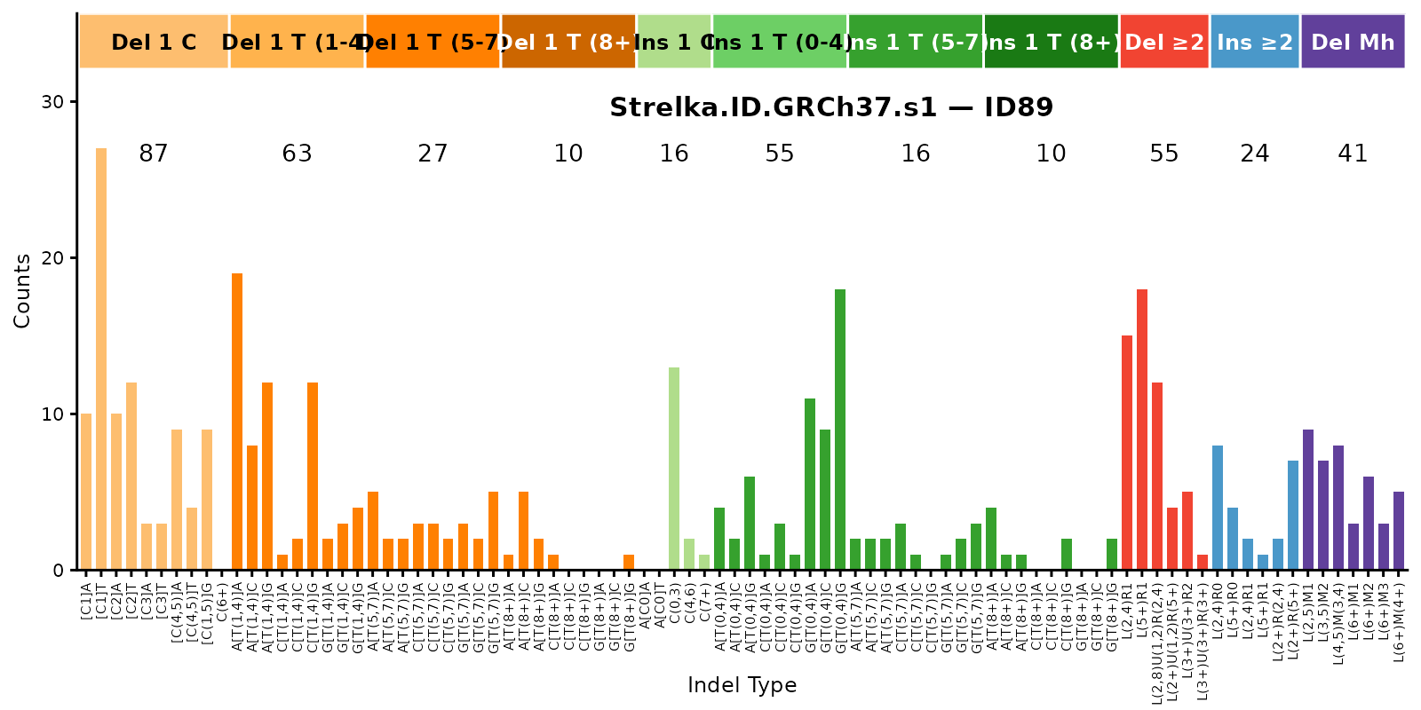
plot_ID476(cat_id476, plot_title = "Strelka.ID.GRCh37.s1 — ID476")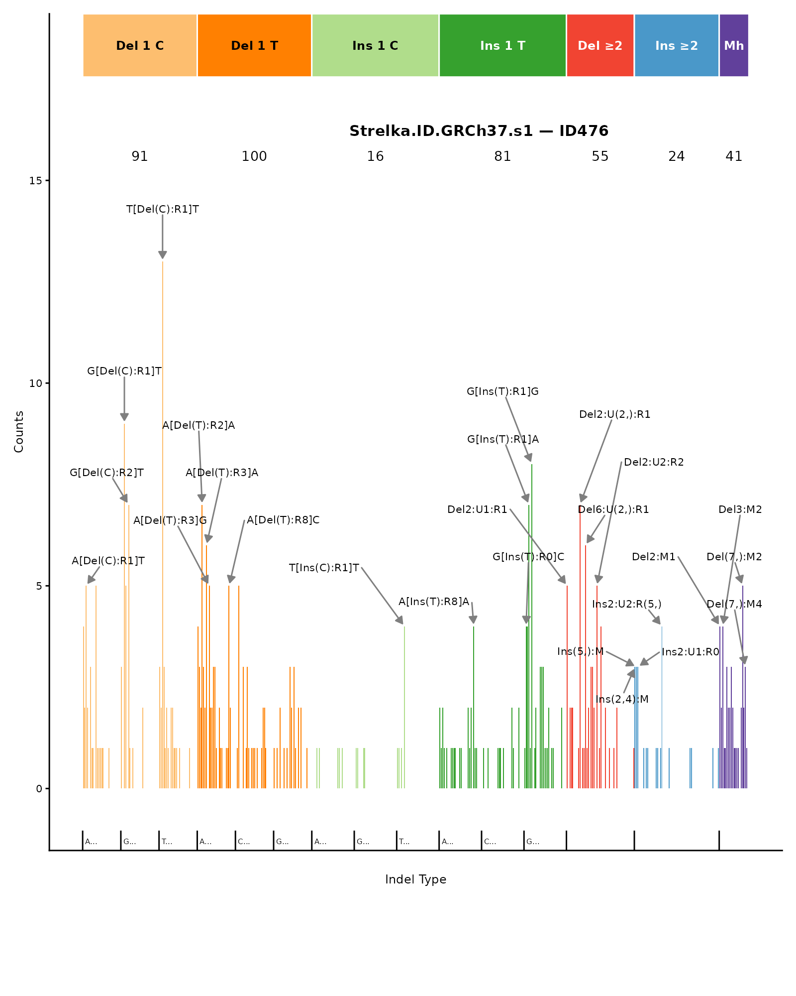
9. Counts ↔︎ density
Convert from raw counts (per category) to mutation density (per megabase of context) using the shipped k-mer abundances:
cat96_density <- transform_catalog(cat96,
                                   target_counts_or_density = "density")
attr(cat96_density, "counts_or_density")
#> [1] "density"
plot_SBS96(cat96_density,
           plot_title = "Strelka.SBS.GRCh37.s1 — SBS96 (density)")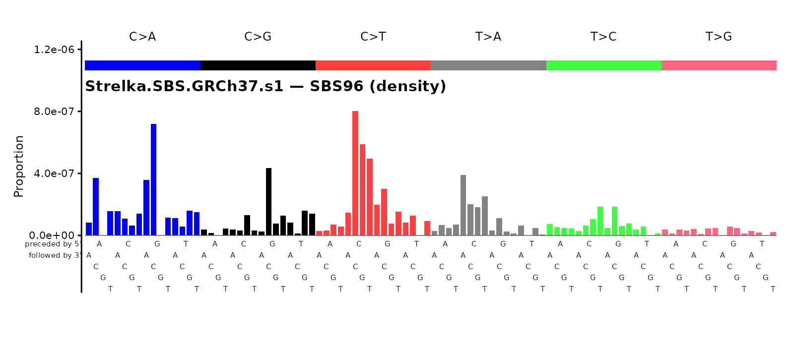
10. Collapse from finer to coarser resolutions
cat96_from_1536 <- collapse_catalog(cat1536, to = "SBS96")
all.equal(as.numeric(cat96_from_1536[, 1]),
          as.numeric(cat96[, 1]))
#> [1] TRUE
11. Catalog I/O
ICAMS-native CSV is the default and only output format today; SigProfiler and COSMIC formats are supported on input.
out_path <- file.path(tempdir(), "Strelka.SBS.GRCh37.s1.SBS96.csv")
write_catalog(cat96, out_path)
cat96_back <- read_catalog(out_path, region = "genome")
identical(as.numeric(cat96), as.numeric(cat96_back))
#> [1] TRUE
See also
-
?read_vcf— the caller-agnostic reader. -
?annotate_sbs_or_dbs_vcf— sequence context + transcript strand for SBS / DBS. -
?annotate_id_vcf— indel justification + classification (COSMIC 83 / Koh 89 / Koh 476) + transcript strand. -
?vcf_to_sbs_catalog,?vcf_to_dbs_catalog,?vcf_to_id_catalog— per-variant-type catalog builders. -
?transform_catalog/?collapse_catalog— counts ↔︎ density and finer-to-coarser collapse. -
?check_and_remove_discarded_variants— optional defensive QC. - The README’s “Gotchas” section documents the cases this pipeline intentionally leaves to the user.